Version: 0.3.38
1. Graph Theory#
- Lecture:
Lecture 6.1
(slides)- Objectives:
Understand what a graph is, what data structures exists to represent it, and when to choose these data structures.
- Concepts:
Graph, path, circuit, edge list, adjacency list, adjacency matrix, depth-first traversal, breadth-first traversal,
We started by looking at sequences, implemented either using arrays or linked lists. In a sequence, each item has at most one predecessor and one successor. We then moved on to trees, where each item can have many successors, but without forming cycles. Graphs generalize these structures: Items can have many successors, many predecessors, cycles, etc. There is no constraint. Fig. 1.15 below illustrates this evolution.

Fig. 1.15 From sequences to graphs, growing data structures in complexity#
Intuitively, a graph is just a collection of “things” linked together in a specific way. In Computer Science (and in Discrete Mathematics), we talk about vertices (singular vertex) connected by edges. Let see what we do with these.
See also
There is no need to become an expert in graph theory. Knowing the basic terminology has however been very useful for me. Here is a reference I used when I need to check something:
📕 Wilson, R. J. (1996). Introduction to graph theory. 4th edition, Addison-Wesley.
Chapters 1 and 2 are already more than what you need to know for this course.
1.1. Graphs in Real-life#
Graph is such a versatile concept. Whatever application domain you work on, there is a graph laying low.
The most obvious example—I believe—comes from transportations. I am sure you have seen buses or subways maps that show how the different lines connect the different stations. The distances are very often inaccurate, but the ordering of stations is enough to find our way. See for instance the Oslo subway map aside on Fig. 1.16. A common problem is thus to find a route between two stations.
Graphs also plays a key role in social media such as Facebook, LinkedIn, Snapchat and the likes. The underlying data model is a simple graph where vertices represent persons, and edges indicate people know one another. The main problems is social network are how many people will my “posts” reach. Who has the most followers, etc?
Internet is another example of “giant” graph. Web sites expose documents that point to other documents using hyperlinks. Here the vertices are the documents and the edges these hyperlinks. Search engines classify web sites according to their visibility, an idea that relates to the probability of a user reaching a web site out of luck. PageRank is one famous such algorithm developed by Google.
Most scientific disciplines use graphs. Electric circuits, which electrical engineers use are also graphs in disguise. Vertices represents electric components such as resistors, lamps, relays, etc., whereas edges represent the wiring. Chemists also rely on graphs to describe chemical compounds: Vertices represents atoms, and edges, bonds. In Biology, graphs describe food-webs, where vertices are animal species and edges denote prey-predator relationship. Public health experts uses graphs to understand how virus propagates through our societies. Vertices are people and edges show the contagion. The same is used by social scientists who study the propagation of ideas. The list goes on and on…
Computer Science is not left out. The flowcharts we have used to visualize algorithms are graphs: Nodes (of various shapes) represent blocks of instructions whereas edges represents the flow of control. In object-oriented analysis, class diagrams (say in UML) are also graphs, where nodes represents classes and edges captures their relationships. Entity-relationships models we use in database are also graphs. You get the idea.
1.2. Graphs Species#
A graph is a very abstract concept: A set of vertices connected by edges. In practice, there are many variations around this theme. Its is important to choose the one that best fit the problem at hand. Let me present the two most common ones, which we will use: Directed and weighted graphs.
1.2.1. Simple Graphs#
The basic form of graph, the simple graph, is a set of vertices and a set of associations between them.
Formally, a simple graph \(G\) is a structure \(G=(V,E)\) where \(V\) is the set of vertices and \(E\) is a set of unordered pairs of vertices, such that \(E \subseteq \{ \, \{x, y\} \, | \, x \in V \, \land \, y \in V \}\).
Consider the “friendship” graph shown below by Fig. 1.17, which portrays a fragment of social network. The persons connected by lines know each other.

Fig. 1.17 A graph connecting people. Edges show who knows who.#
Following the definitions above, we get:
The set of vertices contains all the persons, that is \(V=\{D,E,F,J,L,M,O,P,T\}\).
The set of edges includes 8 unordered pairs \(E=\{ \{D,F\}, \{D,O\}, \{E, O\}, \{F, L\}, \{F, T\}, \{J, L\}, \{J, M\}, \{M, P\}, \{M, O\} \}\).
1.2.2. Directed Graphs#
Sometimes, the relationship between vertices is not symmetrical. In the “friendship” graph above, the “knows” relationship is symmetrical, because we assume that if John knows Lisa, then Lisa knows John too. Contrast this with the food web shown below on Fig. 1.18, where the relationship “preying on” is directed (i.e., not symmetrical). Hawks preys on rabbits, but rabbits do not eat hawks.

Fig. 1.18 A simple “food web” where vertices represents species and arrows represents who eats what.#
We call such graphs directed graphs, by opposition to simple graphs (aka undirected graphs). Formally, a directed graph \(G\) closely resembles a simple graph: It is also a structure \(G=(V,E)\), but E is here a set of ordered pairs such that \(E \subseteq \{ \, (x, y) \, | \, (x,y) \in V^2 \, \}\).
Returning to the food web example from Fig. 1.18, the vertices would be \(V=\{F, G, H, M, R, S \}\) and the edges would be:
1.2.3. Weighted Graphs#
- Sometimes it is necessary to capture a little more about edges and a
straightforward approach is to equip them with a number, which represents a distance, a cost, a likelihood, a capacity, or any other quantity relevant for the problem at hand. This yields a weighted graph. For example, transportation systems often care about the “distance” between two locations (i.e., vertices), as shown on Fig. 1.19 below.

Fig. 1.19 A few Norwegian cities and the road distances that separate them#
Formally, a weighted graph is a structure \(G=(V,E,\phi)\) where \(V\) is the set of vertices, \(E\), the set of edges (directed or not), and \(\phi\) a function that maps every edge to its weight, such that \(\phi : E \to \mathbb{R}\).
Given this definition, the vertex set for the Norwegian cities (see Fig. 1.19) is \(V=\{B, H, M, Op, Os, T, Å\}\), whereas the weight function \(\phi\) would be:
1.2.4. Other Graph Species#
There are a few other species of graph, which we won’t use in this course. I list them below for the sake of completeness.
Multi-graphs are graphs where to vertices can be connected by more than a single edge. The above definition \(G=(V,E)\) falls short in that case, and other mathematical structures are needed, such as the incidence matrix for instance.
Hyper-graphs are graphs where an edge can connect more than two vertices.
Warning
The algorithms and data structures we will study in this course should be adjusted for such more complex species of graph.
1.3. The Graph Jargon#
Besides vertex and edges, there are various terms that carry a specific meaning when it comes to graph theory. Let see the main ones so we can understand what we are talking about..
- walk
A sequence of edges
- path
A walk where every vertex appears only once. In Fig. 1.17 the sequence “Denis, Olive, Mary” is a path.
- cycle
A walk that starts where its ends. In Fig. 1.17 the sequence “Denis, Olive, Mary, John, Lisa, Frank, Denis” is a cycle
- loop
An edge whose two members are the same vertex. There is no such a loop on Fig. 1.17.
- adjacent vertices
Two vertices are adjacent if there exists an edge that connects them. Denis is only adjacent to Frank and Olive.
- incident edge (to a vertex)
An edge is incident to a vertex it connects to or from this vertex.
- degree (of a vertex \(v\))
The number of edges that are incident to Vertex \(v\). A vertex of degree zero is called an isolated vertex, and a vertex of degree 1 is an end-vertex. For directed graphs, the in-degree and out-degree are the numbers of edges to and from, respectively.
- connected graph
A graph where every two vertices are connected by a path.
- subgraph
A subgraph of a graph \(G=(V,E)\), is another graph \(G'\) whose vertices and edges are all included in \(V\) and \(E\), respectively. The vertex set of \(G'\) has to contain the subset of vertices incident to the selected edges.
- component
A “maximum” connected subgraph, that is connected subgraph, to which one cannot add any vertex without loosing the “connectivity” property
- complete graph
A graph where every pair of vertex is adjacent
- regular graph
A graph where every vertex has the same degree
- tree
An undirected graph that has no cycle and where every pair of vertex is connected by exactly one path.
- forest
An undirected graph that has no cycle and where every pair of vertex is connected by at most one path. In other words, a forest is a graph where every component is a tree.
1.4. Alternative Representations#
So far we have defined a graph by its list of edges, that is a structure \(G=(V, E)\), where \(V\) is a set of vertices and \(E\) is the set of edges. At times, other “representations” come up handy, namely the adjacency matrix and the incidence matrix.
1.4.1. Adjacency Matrix#
The adjacency matrix \(A\) is an \(|V| \times |V|\) matrix where the cell \(c_{ij}\) contains the number of edges between vertices \(i\) and \(j\). The adjacency matrix is, by definition, a square matrix.
Consider again the friendship graph shown above on Fig. 1.17. Provided we number the vertices \(V=\{D,E,F,J,L,M,O,P,T\}\) in alphabetical order, the adjacency matrix would be:
1.4.2. Incidence Matrix#
When edges have their own identity, we can use an incidence matrix, which maps every vertex onto its incident edges. The incidence matrix is therefore an \(|V| \times |E|\) matrix \(I\), such that every cell \(c_{i,j}\) is 1 if an only if Vertex \(v_i\) is incident to Edge \(e_j\). If the graph is directed, the cell \(c_{i,j}\) can contains -1 if the vertex is the source, 1 if the vertex is the target and 0 otherwise. This is one way to capture multi-graphs and/ hyper-graphs for instance.
Look again at Fig. 1.18, the dummy food web. Provided that vertices and edges are ordered alphabetically, the incidence matrix \(I\) would be:
1.5. Graph Problems#
There are many graph problems that arises from the graph structure. Many of them are “difficult”, that is, for we only know “inefficient algorithms” (i.e., of exponential complexity). Here is a few well known examples:
- Hamiltonian Path
Find a Hamiltonian path in a graph, that is a path that visits every vertex only once.
- Shortest path
Find the shortest path between two vertices in a weighted graphs. We will look at three algorithms to tackle this, namely Dijkstra, Bellman-Ford, and Floyd-Warshall.
- Traveling Salesperson Problem (TSP)
Given a weighted graph, find the shortest cycle that visits all the vertices.
- Graph Coloring
Find a mapping from the set of vertices to a given set of colors, such that there is no two adjacent vertex that map to the same color.
- Minimum Spanning Tree (MST)
Given a weighted graph, find the tree that covers all the vertices and has the minimum total weight.
- Cycle Detection
Find cycles in a given graph.
- Vertex cover
Given a graph G=(V,E), find a subset of vertices V’ such that every edges is incident to an vertex in V’.
- Independent set
Given a graph G=(V,E), find a subset of vertices V’ such that no vertex in V’ is adjacent to a vertex in V.
1.6. Graphs as Data Structures#
Besides being a mathematical concept, a graph is also a data structure. Intuitively, the queries one runs against a graph include:
1.6.1. Graph ADT#
There is no agreement on what the graph abstract data type should be. There are indeed many operations that one can perform on a graph, finding cycles, components, unreachable vertices, etc. Graphs are highly application dependent. I put below what seems to me like a common minimal set of operations:
- empty
Create a new empty graph, that is an graph with no vertex or edge.
- add vertex
Add a new vertex to the given graph. What identifies the vertex, as well as the information its carries depend on the problem and or the selected internal representation.
- remove vertex
Delete a specific vertex from the given graph. Either this raises an error if the selected vertex still has incoming or outgoing edges, or it removes these edges as well.
- add edge
Create a new edge between the two given vertices. What identifies this edge as well as the information it carries depend on the problem and the chosen internal representation.
- remove edge
Remove the selected edge.
- edges from
Returns the list of edges whose source is the given vertex
- edges to
Returns the list of edges whose target is the given vertex
- is_adjacent
True if an only if there exist an edge between the two given vertices
1.6.2. Graph Representations#
There are many ways to implement the graph ADT above, from a simple list of edges to more complicated structures using hashing. As always, the one to use depends on the problem at hand. Let see the most common ones.
In the general case, there is some information attached to either the vertex, the edges, or to both. The internal representation we choose impact however the implementation (and the efficiency) of the operations.
Operations |
Edge List |
Adjacency List |
Adjacency Matrix |
|---|---|---|---|
add vertex |
O(1) |
O(1) |
|
remove vertex |
O(V) |
O(V) |
|
add edge |
O(1) |
O(1) |
|
remove edge |
O(E) |
O(V+E) |
|
edges from |
O(E) |
O(deg(v)) |
|
edges to |
O(E) |
O(deg(v)) |
|
is adjacent |
O(E) |
O(1) |
1.6.2.1. Edge List#
The simplest solution is simply to store a sequence of edges, where each edge includes a source vertex, a target vertex and a label. With this design a vertex is identified by its index in the underlying list of vertices, and an edge by its index in the underlying list of edges.

Fig. 1.20 Overview of an edge list implementation. Vertices and edges are records, stored into separate sequences.#
While simple, the main downside of this scheme is that most of
operations on graphs rely on linear search to find either the vertex
or the edge of interest. Listing 1.11 illustrates this
issue on the edgesFrom method, where we have to iterate through
all the edges to find those whose source vertex match the given one.
public class EdgeList<V, E> {

   class Edge {
      private int source;
      private int target;
      private E label;
   }

   private List<V> vertices;
   private List<Edge> edges;

   public List<Integer> edgesFrom(int source) {
       final var result = new ArrayList<Integer>();
       for(var edge: this.edges) {
          if (edge.source == source) {
             result.add(edge);
          }
       }
       return result;
   }

   // Etc.
}
1.6.2.2. Adjacency List#
Another possible representation is the adjacency list: Each vertex gets its own list of incident edges. Often, store a hash table to retrieve specific vertex faster. When edges have no label/payload, each vertex is associated with the list of adjacent vertices (so the name “adjacency list”).
The benefit of the this adjacency list is that is speed up the retrieval of incoming and outgoing edges. These are often very useful operation, for example, to traverse the graph (see Graph Traversals)
public class AdjacencyList<V, E> {

   class Edge {
      int source;
      int target;
      E payload;

      // etc.
   }

   class Vertex {
      V payload;
      List<Edge> incidentEdges;

      // etc.
   }

   private List<Vertex> vertices;
   private List<Edge> edges;

   public List<Integer> edgesFrom(int source) {
       final var result = new ArrayList<Integer>();
       for(var edge: this.vertices[source].incidentEdges) {
          if (edge.source == source) {
             result.add(edge);
          }
       }
       return result;
   }

   // etc.
}
1.6.2.3. Adjacency Matrix#
Note
Graphs can quickly become very large. Take social media for instances with millions of users, or package dependencies in Python of JavaScript. Such large graphs requires dedicated storage solution, more like databases. Relational databases such as MySQL are however inappropriate and dedicated solution exists such as such as Neo4j for instance.
1.6.3. Graph Traversals#
As we have seen for trees, one may need to navigate through the structure of the graph, for instance to find whether there is a path between two vertices.
We can adapt the two traversal strategies we have studied for trees, namely, the breadth-first and the depth-first traversal. The only difference is that graphs may contain cycles, and that we remember which vertices we have already “visited” to avoid “looping” forever in a cycle.
As we progress through a graph we need to keep track of two things:
The vertices that we have discovered but not yet processed. We will name these
pendingverticesThe vertices that we have already visited (i.e., processed). We will name these the
visitedvertices.
1.6.3.1. Depth-first Traversal#
Intuitively, a depth-first traversal never turns back, except once it reaches a dead-end, either because the vertex it has reached has no outgoing edge, or because it has already “visited” all the surrounding vertices. The depth-first traversal would proceed as follows:
Add the entry vertex to the sequence of pending vertices
While there are pending vertices,
Take out the last pending vertex added
If that vertex is not in the set of visited ones
Add it to the set of visited vertices
Add all vertices that can be reached from there
depth_first_alg below shows a Java implementation of this
algorithm. Note the use of a stack (see Line 3) which forces the
extraction of the last inserted pending vertex.
 1public void depthFirstTraversal(Graph graph, Vertex entry) {
 2   final var visited = new HashSet<Vertex>();
 3   final var pending = new Stack<Vertex>();
 4   pending.push(entry);
 5   while (!pending.isEmpty()) {
 6       var current = pending.pop();
 7       if (!visited.contains(current)) {
 8           System.out.println(current);
 9           visited.add(current);
10           for (var eachEdge: graph.edgesFrom(current)) {
11               pending.push(eachEdge.target)
12           }
13       }
14   }
15}
Consider for example depth_first_example below, which shows
a “friendship” graph. Vertex represent persons, whereas an edge between two
persons indicates they know each other. Edges are bidirectional and
can be navigated both ways. Starting from “Denis”, this depth-first
traversal will reach the vertices in the following order: Denis,
Frank, Lisa, John, Mary, Olive, Erik, Peter, and Thomas.
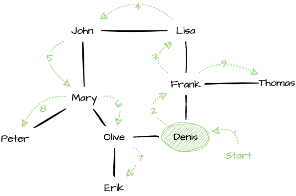
Fig. 1.21 Traversing a graph “depth-first”, starting from the vertex “Denis” (assuming neighbors are visited in alphabetical order). This yields the following order: Denis, Frank, Lisa, John, Mary, Olive, Erik, Peter, Thomas.#
Let see how the visited and pending variables evolve in this
example.
Step |
Current |
Pending |
visited |
See lines |
|---|---|---|---|---|
0 |
\(D\) |
\(()\) |
\(\{\}\) |
Line 6 |
1 |
\(D\) |
\(()\) |
\(\{D\}\) |
Line 9 |
2 |
\(D\) |
\((O,F)\) |
\(\{D\}\) |
Line 10-12 |
3 |
\(F\) |
\((O)\) |
\(\{D\}\) |
Line 6 |
4 |
\(F\) |
\((O)\) |
\(\{D,F\}\) |
Line 9 |
5 |
\(F\) |
\((O,T,L,D)\) |
\(\{D,F\}\) |
Line 10-12 |
6 |
\(D\) |
\((O,T,L)\) |
\(\{D,F\}\) |
Line 6 |
7 |
\(L\) |
\((O,T)\) |
\(\{D,F\}\) |
Line 6 |
8 |
\(L\) |
\((O,T)\) |
\(\{D,F,L\}\) |
Line 9 |
9 |
\(L\) |
\((O,T,J,F)\) |
\(\{D,F,L\}\) |
Line 10-12 |
10 |
\(F\) |
\((O,T,J)\) |
\(\{D,F,L\}\) |
Line 6 |
11 |
\(J\) |
\((O,T)\) |
\(\{D,F,L\}\) |
Line 6 |
12 |
\(J\) |
\((O,T)\) |
\(\{D,F,J,L\}\) |
Line 9 |
13 |
\(J\) |
\((O,T,M,L)\) |
\(\{D,F,J,L\}\) |
Line 10-12 |
14 |
\(L\) |
\((O,T,M)\) |
\(\{D,F,J,L\}\) |
Line 6 |
15 |
\(M\) |
\((O,T)\) |
\(\{D,F,J,L\}\) |
Line 6 |
16 |
\(M\) |
\((O,T)\) |
\(\{D,F,J,L,M\}\) |
Line 9 |
17 |
\(M\) |
\((O,T,P,O,J)\) |
\(\{D,F,J,L,M\}\) |
Line 10-12 |
18 |
\(J\) |
\((O,T,P,O)\) |
\(\{D,F,J,L,M\}\) |
Line 6 |
19 |
\(O\) |
\((O,T,P)\) |
\(\{D,F,J,L,M\}\) |
Line 6 |
20 |
\(O\) |
\((O,T,P)\) |
\(\{D,F,J,L,M,O\}\) |
Line 9 |
21 |
\(O\) |
\((O,T,P,M,E,D)\) |
\(\{D,F,J,L,M,O\}\) |
Line 10-12 |
22 |
\(D\) |
\((O,T,P,M,E)\) |
\(\{D,F,J,L,M,O\}\) |
Line 6 |
23 |
\(E\) |
\((O,T,P,M)\) |
\(\{D,F,J,L,M,O\}\) |
Line 6 |
24 |
\(E\) |
\((O,T,P,M)\) |
\(\{D,E,F,J,L,M,O\}\) |
Line 9 |
25 |
\(E\) |
\((O,T,P,M,O)\) |
\(\{D,E,F,J,L,M,O\}\) |
Line 10-12 |
26 |
\(O\) |
\((O,T,P,M)\) |
\(\{D,E,F,J,L,M,O\}\) |
Line 6 |
27 |
\(M\) |
\((O,T,P)\) |
\(\{D,E,F,J,L,M,O\}\) |
Line 6 |
28 |
\(P\) |
\((O,T)\) |
\(\{D,E,F,J,L,M,O\}\) |
Line 6 |
29 |
\(P\) |
\((O,T)\) |
\(\{D,E,F,J,L,M,O,P\}\) |
Line 9 |
30 |
\(P\) |
\((O,T,M)\) |
\(\{D,E,F,J,L,M,O,P\}\) |
Line 10-12 |
31 |
\(M\) |
\((O,T)\) |
\(\{D,E,F,J,L,M,O,P\}\) |
Line 6 |
32 |
\(T\) |
\((O)\) |
\(\{D,E,F,J,L,M,O,P\}\) |
Line 6 |
33 |
\(T\) |
\((O)\) |
\(\{D,E,F,J,L,M,O,P,T\}\) |
Line 9 |
34 |
\(T\) |
\((O,F)\) |
\(\{D,E,F,J,L,M,O,P,T\}\) |
Line 10-12 |
35 |
\(F\) |
\((O)\) |
\(\{D,E,F,J,L,M,O,P,T\}\) |
Line 6 |
36 |
\(O\) |
\(()\) |
\(\{D,E,F,J,L,M,O,P,T\}\) |
Line 6 |
1.6.3.2. Breadth-first Traversal#
The breadth-first traversal closely resembles the depth-first traversal, but instead of pushing on forward until a dead-end, it systematically explores all children, levels by levels. First, the adjacent vertices, then the vertices two edges away, then those three edges away, etc. It could be summarized as follows:
Add the entry vertex to the pending vertices
While there are pending vertices,
Pick the first pending vertex (by order of insertion)
If that vertex has not already been visited
Mark it as visited
Add to pending vertices, all vertices that can be reached from that vertex
The only difference with the depth-first traversal is the element we pick from the list of pending vertices: The breadth-first traversal uses the first inserted, whereas the depth-first traversal uses the last inserted.
breadth_first_java below illustrates how a breadth-first
traversal could look like in Java. We use a Queue to ensure we
always pick the first pending vertex, by insertion order.
 1public void breadthFirstTraversal(Graph graph, Vertex entry) {
 2   final var visited = new HashSet<Vertex>();
 3   final var pending = new Queue<Vertex>();
 4   pending.push(entry);
 5   while (!pending.isEmpty()) {
 6       var current = pending.remove(0);
 7       if (!visited.contains(current)) {
 8           System.out.println(current);
 9           visited.add(current);
10           for (var eachEdge: graph.edgesFrom(current)) {
11               pending.push(eachEdge.target)
12           }
13       }
14   }
15}
Consider again the “friendship” graph introduced in above in
depth_first_example and reproduced below on
breadth_first_example. A breadth-first traversal starting
from “Denis” proceeds by “levels”. First it looks at all the adjacent
vertices, namely Frank and Olive. Then, it looks at vertices that it
can reach from those, that is Lisa, Thomas, Mary, and Olive. And then
it continues exploring nodes one more edge away, namely John and
Peter.

Fig. 1.22 Traversing a graph “breadth-first”. It enumerates vertices by “level”, as follows: Denis, Frank, Olive, Lisa, Thomas, Erik, Mary, John, Peter.#