Version: 0.3.38
3. Using Dynamic Arrays#
- Lecture:
Lecture 2.3
(slides)- Objectives:
Understand amortized analysis and dynamic arrays
- Concepts:
Amortized analysis, dynamic arrays, memory allocation
In the previous lecture, we implemented our sequence ADT using an array. We overlooked however the infinite nature of sequences1In maths, sequences are possibly infinite. Consider for instance the sequence of prime numbers or the Fibonacci sequence. and we implemented instead fixed-capacity sequences. We will do better here. While looking at the runtime efficiency of the insertion and deletion, we shall introduce amortized analysis.
3.1. Infinite Sequences#
So far implementation of the sequence ADT uses a fixed capacity. Each sequence we create can contain a predefined number of items. How can we work around this and create sequences that hold as many items as we need. I reproduce below the code we used for the insertion:
void
seq_insert(Sequence* sequence, void* item, int index) {
  assert(sequence != NULL);
  assert(sequence->length < CAPACITY);
  assert(index > 0 && index <= sequence->length + 1);
  for (int i=sequence->length ; i>=index ; i--) {
    sequence->items[i+1] = sequence->items[i];
  }
  sequence->items[index] = item;
  sequence->length++;
}
What would happen if we exceed that capacity? Consider for instance
the code below, where we create a sequence and then insert() 200
times at the end.
#include <stdio.h>
#include "sequence.h"

int main(int argc, char** argv) {
  Sequence* seq = seq_create();
  int test = 23;
  for (int i=0 ; i<200 ; i++) {
    printf("%d ", i);
    seq_insert(seq, (void*) &test, seq_length(seq) + 1);
  }
  printf("Done.\n");
}
The assertion we placed in the insert() fails as soon as the
given position exceeds the capacity and the program terminates with an
error.
Can we do better? Yes, when there is not enough capacity, we need to a bigger array, copy what is already in our array, and finally release our previous array. Similarly, when there is too much unused capacity, we can allocate a smaller array, copy the current items, and finally release our big unused array.
Caution
This data structure, where we dynamically allocate a new array when the current one is too small (or too large) is often referred to as dynamic arrays. There are other names however such as “array lists” or “re-sizable arrays”. As often, there is no clear consensus.
3.1.1. Memory Representation#
As opposed to our fixed-capacity implementation, we need to store the capacity of the sequence into our record. We can simply update our C structure as follows:
struct sequence_s {
  int    capacity; // The current capacity
  int    length;
  void** items;
};
With this new memory representation, we have to update our
implementation of the create() operation as follows. We need to
initialize the value of our new capacity field, and allocate the
arrays of items accordingly.
const int INITIAL_CAPACITY = 10;

Sequence* seq_create(void) {
  Sequence* new_sequence = malloc(sizeof(Sequence));
  new_sequence->capacity = INITIAL_CAPACITY;
  new_sequence->length   = 0;
  new_sequence->items    = malloc(INITIAL_CAPACITY * sizeof(void*));
  return new_sequence;
}
3.1.2. Insertion#
Now we can modify our implementation of the insert()
operation. If the given sequence is “full”, we need to “resize it”.
To detect whether a sequence is “full”, we compute its load factor, as the ratio between its length and its capacity. For instance, if the length is 5 and the capacity is 10, the load will be 0.5. Similarly, if the length is 3 and the capacity is 12, the load is 0.25. We simply use a load threshold to decide whether or not to resize the underlying array.
 1const double GROWTH_THRESHOLD = 1.0;
 2const double GROWTH_FACTOR = 2.0;
 3
 4void
 5seq_insert(Sequence* sequence, void* item, int index) {
 6  assert(sequence != NULL);
 7  assert(index > 0 && index <= sequence->length + 1);
 8  if (load_factor(sequence) >= GROWTH_THRESHOLD) {
 9    resize(sequence, GROWTH_FACTOR);
10  }
11  for (int i=sequence->length ; i>=index ; i--) {
12    sequence->items[i+1] = sequence->items[i];
13  }
14  sequence->items[index] = item;
15  sequence->length++;
16}
17
18double
19load_factor(Sequence* sequence) {
20  assert(sequence != NULL);
21  return sequence->length / sequence->capacity;
22}
To resize the underlying array by a given factor, we proceed as follows:
We compute the new capacity
We allocate a new array with the new capacity
We copy all the existing items from the “old” array into the new array
We attach the new array to the sequence’s record
We free the old array
void
resize(Sequence* sequence, double factor) {
  assert(sequence != NULL);
  assert(factor > 0);
  if (sequence->capacity > 1 || factor >= 1) {
    sequence->capacity = (int) sequence->capacity * factor;
    void** old_array = sequence->items;
    void** new_array = malloc( sequence->capacity * sizeof(void*));
    for(int i=0 ; i<sequence->length ; i++) {
      new_array[i] = old_array[i];
    }
    free(old_array);
    sequence->items = new_array;
  }
}
3.1.3. Deletion#
We also have to adjust the deletion and shrink the array when the load factor drops below a chosen shrink threshold. We can reuse the same resize helper, but pass it a fraction such as 1/2 to halve the array. The rest remain the very same than for the fixed-capacity sequences.
const double SHRINK_THRESHOLD = 0.5;
const double SHRINK_FACTOR = 0.5;

void
seq_remove(Sequence* sequence, int index) {
  assert(sequence != NULL);
  assert(index > 0 && index <= sequence->length + 1);
  if (load_factor(sequence) < SHRINK_THRESHOLD) {
    resize(sequence, SHRINK_FACTOR);
  }
  for(int i=index ; i<sequence->length ; i++) {
    sequence->items[i] = sequence->items[i+1];
  }
  sequence->items[sequence->length] = NULL;
  sequence->length--;
}
3.2. Runtime Analysis#
In such dynamic arrays, resizing does not always happen, but only when it gets full. Many data structures behave that way, doing some house-cleaning in some specific situations. Let’s see where the techniques we have studied so far fall flat.
3.2.1. Best-case Scenario#
Consider again our insertion algorithm (see Listing 3.7) that allocates a new array when the existing one is full. What is the best-case scenario?
The best case (for any sequence of a given length) implies that:
The array is not full, so there is no extra work to re-allocate and copy the existing items
The insertion occurs at the end of the sequence so there is no shifting of the existing items.
When these two conditions are met, our insertion runs in constant runtime \(O(1)\). Table 3.2 details how to count the operations our insertion performs. In the best-scenario it always performs 6 operations (a constant).
Line |
Fragment |
Cost |
Runs |
Total |
|---|---|---|---|---|
8 |
|
2 |
1 |
2 |
9 |
|
n |
0 |
0 |
11 |
|
1 |
1 |
1 |
11 |
|
1 |
1 |
1 |
11 |
|
1 |
0 |
0 |
12 |
|
2 |
0 |
0 |
14 |
|
1 |
1 |
1 |
15 |
|
1 |
1 |
1 |
Total: |
6 |
3.2.2. Worst-case Scenario#
The worst-case scenario (for any sequence of a given length) implies that:
The array is full and we need to resize it before to proceed with the insertion per se.
The insertion targets the first position, so the whole underlying array has to be shifted forward.
When these two conditions are met, our instertion algorithm (see Listing 3.7) runs in \(O(n)\). Table 3.3 details how we get so this results.
Line |
Fragment |
Cost |
Runs |
Total |
|---|---|---|---|---|
8 |
|
2 |
1 |
2 |
9 |
|
n |
1 |
n |
11 |
|
1 |
1 |
1 |
11 |
|
1 |
n+1 |
n+1 |
11 |
|
2 |
n |
2n |
12 |
|
2 |
n |
2n |
14 |
|
1 |
1 |
1 |
15 |
|
2 |
1 |
2 |
Grand Total: |
6n+7 |
|||
3.2.3. Average-case Scenario#
What about the average scenario. If we assume nothing about the given scenario, in average it depends on two things:
Do we need to resize the underlying array (see Line 8 in Listing 3.7).
Where do we insert in the array? The closer to the end of the array, the less work we do.
If we want to formalize this, we need to define two random variables that captures these situation. Let’s go:
\(F\) capture whether the array if full or not. It takes two values, either 0 or 1, with equal probability.
\(C\) captures where we need to insert in the array. It takes any value in the interval \([1, n+1]\).
We can modify our calculation accordingly to reflect these two, as shown in In Table 3.4
Line |
Fragment |
Cost |
Runs |
Total |
|---|---|---|---|---|
8 |
|
2 |
1 |
2 |
9 |
|
n |
F |
\(nF\) |
11 |
|
1 |
1 |
1 |
11 |
|
1 |
C+1 |
\(C+1\) |
11 |
|
1 |
C |
\(C\) |
12 |
|
2 |
C |
\(2C\) |
14 |
|
1 |
1 |
1 |
15 |
|
1 |
1 |
1 |
Total: |
\(nF + 4C + 6\) |
To complete our calculation, we need to factor in the probability that these two random variables take specific values. We thus compute the expected value of the function \(f(n,F, C)=nF + 4C + 6\), which yields \(2.5n + 10\)
Detailed Calculation of \(E[f(n,F,C)]\)
Since \(F\) only takes two values 0 or 1, we can further break this expression:
We can look at each of the two sums in turn. We know that c takes values in the interval \([1, n+1]\), that gives us:
We can proceed similarly with the second sum:
We can now put everything together as follows:
3.3. Amortized Analysis#
The analysis we run above describe inserting into a random sequence. In practice however, this seldom happen. The common use-case is to create a sequence and then to insert, delete, etc. in it.
Consider again our insertion algorithm. We do not resize all the time, but only when it gets full. Say we start with an empty array of 2 cells and we double it only when it gets completely full. Then, only the second, fourth, eighth, sixteenth, etc. would require extra “resizing” work. Amortized analysis captures the average cost over a sequence of insertion. Fig. 3.5 illustrates this behavior.
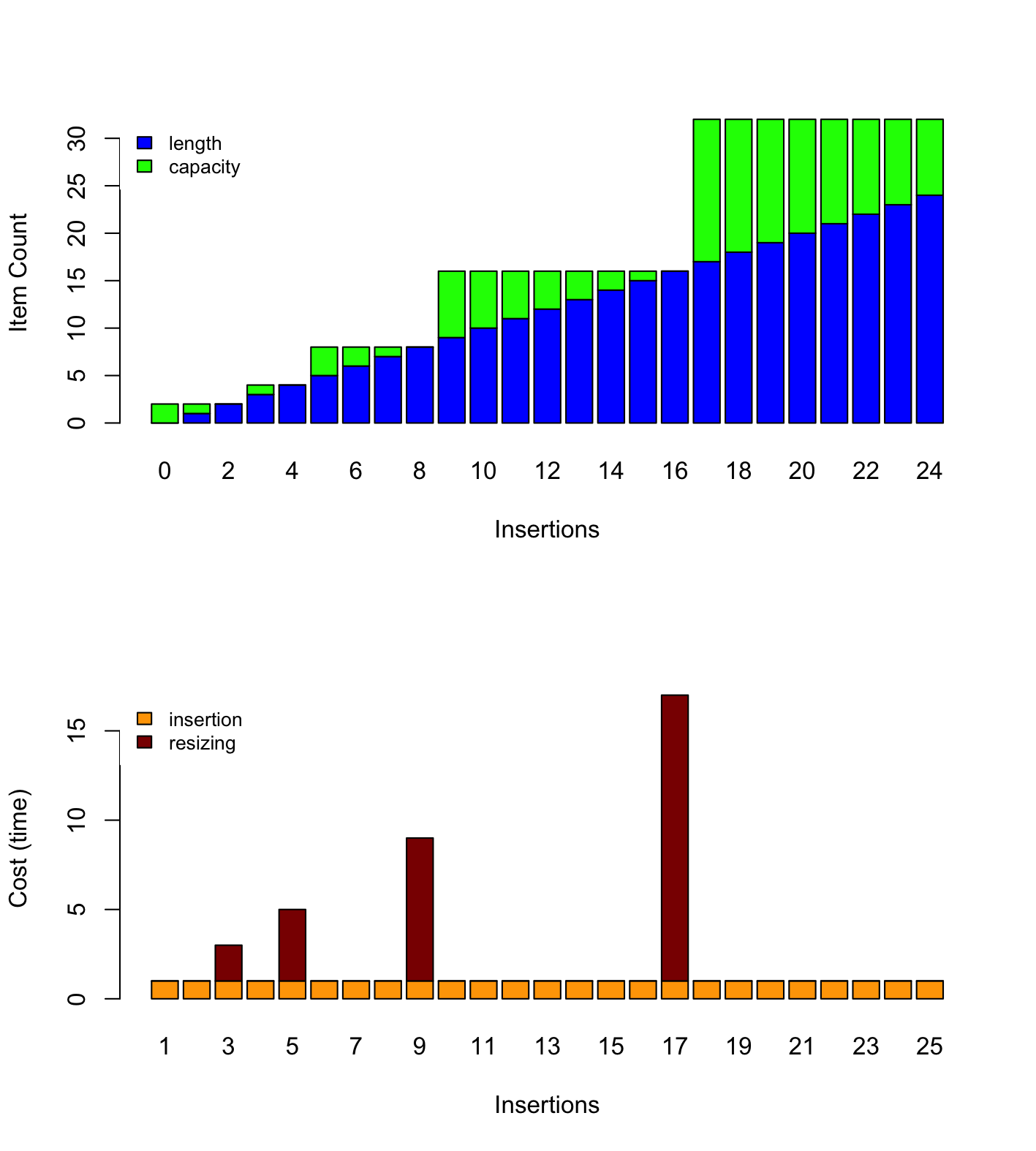
Fig. 3.5 Behavior and cost of the insertion using a dynamic array#
In other words, amortized analysis tells us the average cost over a many insertions.
There are three main “methods” to approach amortized analysis:
The Aggregate Method, often useful for understanding the concept on simple cases
The Banker Method that applies to more complex cases
The Physicist Method, which is alternative which also can be used on complex cases.
Important
Amortized Analysis vs. Average-case Analysis
Average case analysis focuses on algorithms regardless of any data structures. By contrast, amortized analysis focuses on how algorithms perform while used repeatedly for a single data structure.
3.3.1. The Aggregate Method#
As we have just seen, amortized analysis tells us the average cost over a sequence of operations applied to single data structure. The aggregate method implements this idea by computing this average explicitly. Provided that the cost of a single operation is \(t(n)\), the aggregate method computes an average cost \(t^*(k)\) as follows:
Visually, this means computing the average of the bars shown on Fig. 3.5.
Aggregate Method, Detailed Calculation
For the sake of simplicity, let’s assume the insertion cost 1 unit of time when we do not need to resize. That gives us a simpler cost function \(t(n)\) such as:
Now, using the aggregate methods, we need to compute average value of \(t(n)\) when \(n\) grows. As shown in Fig. 3.5, if we perform \(k\) insertions on the same, then there will be \(\left \lfloor \log_2 k \right \rfloor\) resizings (each that costs n). The “trick”, is that we can sum the insertions and the resizings separately (see the orange and red blocks on Fig. 3.5).
The aggregated cost, which we denote by \(t^*(k)\) is therefore:
As shown below, we can see that the function \(t^*(k) = \frac{3k-2}{k}\) tends towards 3 as k tends towards infinity. We can conclude that this function is bounded above by a constant (i.e., 3), that is \(t^*(k) \in O(1)\).
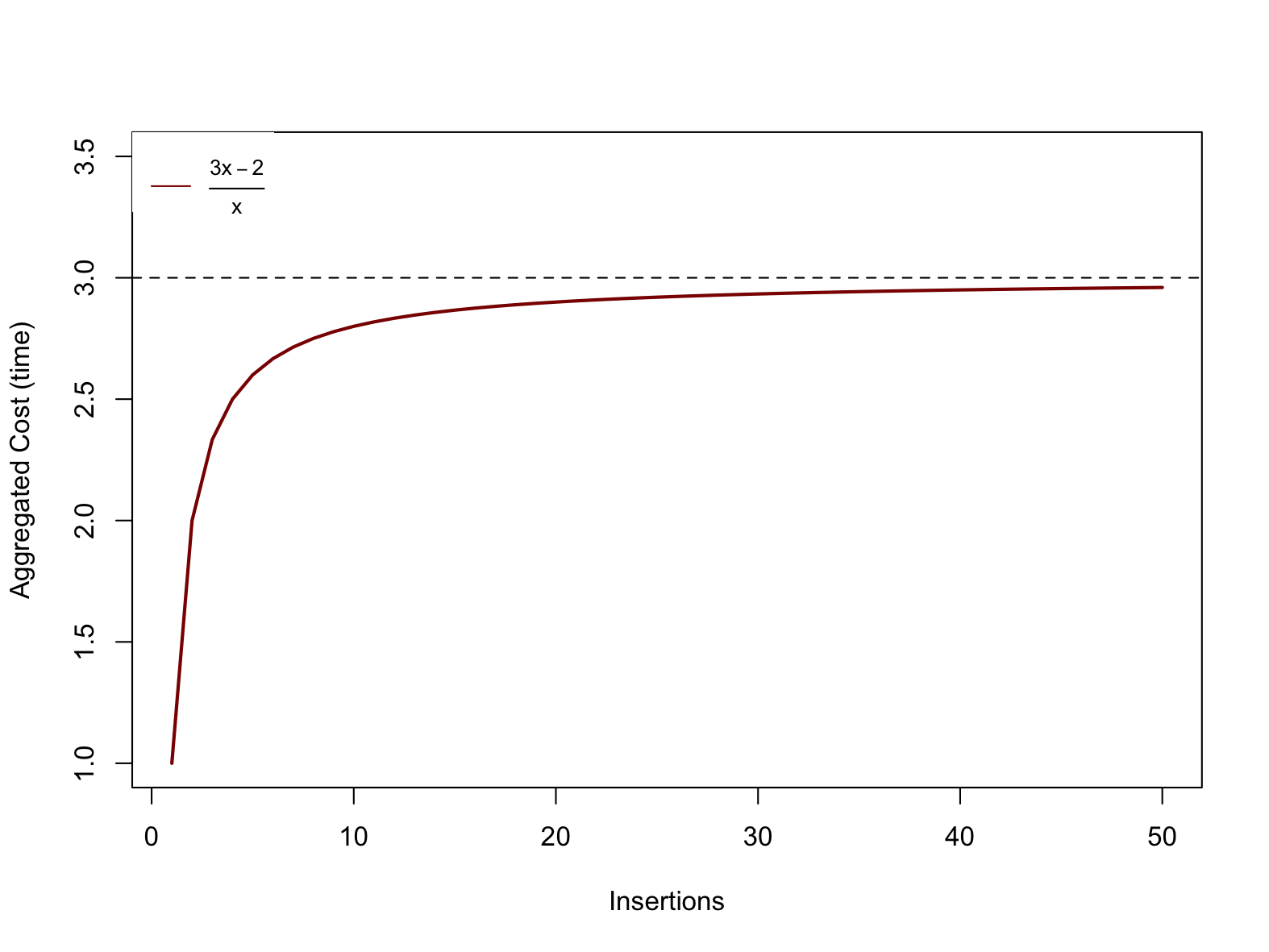
Fig. 3.6 \(f(x) = \frac{3x-2}{x}\) tends towards 3 as \(x\) grows.#
3.3.2. The Banker Method#
The banker methods takes a different road, but the aims is the same: Estimate the average cost of a sequence of operations applied to a single data structure.
The banker methods follows an analogy where costs are spent money. The intuition is that instead of spending very little “money” on most insertions, but much more on those few that require resizing, the banker method imagines accumulating some extra “money” in a piggy bank, which we could later use to compensate when a resizing is needed. The challenge is to find how much we should save in our piggy bank each time, so that we never run out of money.
The banker money aims at proving that there exists a small amount (often a constant), which we can save every time and that would compensate when expensive operations later occur. To prove that, we proceed with induction in two steps:
Show that given a starting amount of money (our initial deposit), and a fix saving, we can “pay for” the first expensive operation.
Show that provided our balance was positive after an expensive operation, we will accumulate enough and “pay for” the next expensive operation.
Detailed proof using the Banker method
Consider again that we “double” the capacity array, when it is exactly full. If we start with an empty array of length 2, and if we assume that at every operation, we put 2 units in our piggy bank. How to prove that this is enough?
First we must prove that our saving of two units will cover the first expensive operation, which occurs during the third insertion, we we must copy the existing 2 buckets. Intuitively, it works: We are left with 4 in our bank, since we collect \(3 \times 2\) in our bank and pay 2. For this we can expand the first few steps, as done below in Table 3.5.
Table 3.5 Expanding the first few insertions# Insertion
Length
Capacity
Saving
Resizing Cost
Balance
0
0
2
NA
NA
0
1
1
2
2
0
2
2
2
2
2
0
4
3
3
4
2
2
4
Then, we have to prove that if we have a non negative balance after a insertion that triggers a resizing, we will collect enough to pay for the next resizing.
Note that resizing occurs at every insertion that of the form \(2^k + 1\), that is 3, 5, 9, 17, 33, etc. At each of these resizings, we must pay \(2^k\). So we must then prove that if our balance \(b\) is 0 (non-negative), after resizing \(k\), the balance \(b'\) after resizing k+1 is also positive.
\[\begin{split}b' &= \left[2 \cdot \left( (2^{k+1} + 1) - (2^{k} + 1) \right) \right] - 2^{k} \\ &= 2^{k+2} + 2 - 2^{k+1} - 2 - 2^k \\ &= 2^{k+2} - 2^{k+1} - 2^{k} \\ &= 2^{k} \cdot (2^2 - 2^1 - 1) \\ &= 2^{k}\end{split}\]
We can thus conclude that the cost of resizing is nothing more than an extra constant cost of 2, that is the resizing has a constant amortized cost.
3.4. Summary#
We have improved our implementation of the sequence ADT by removing of the fixed capacity, and resizing the underlying array when it needed.
This resizing operation occurs only when the array is too full (resp. too empty) and calls for a new type of analysis: amortized analysis, which looks at the average cost of sequences of operations on a single data structure . We looked into two methods: the aggregate method and the banker’s method.